Since February 2016, I have been participating in DIYRobocars meetups here in the SF Bay Area, wherein a bunch of amateur roboticists compete in autonomous time trials with RC cars. I had been doing very well in the competition with essentially just a glorified line-following robot, but have lately upgraded to a full SLAM-like approach with a planned trajectory.
In this series of posts I will try to brain-dump everything I’ve learned in the last two years, and explain how my car works.
In part 1, I covered some basic control strategies. In this part, I’ll discuss how to determine the car’s position relative to the line (or vice versa).
Tracking lane lines
In the previous part, I mentioned the curvilinear coordinate system that a line-tracking car lives in:

Once we know \(y\), \(\psi\), and \(\kappa\), we can apply the control strategies from part 1.
Finding lane lines in an image
This is a pretty well-studied problem at this point. The fixme add links Udacity self-driving course walks you through a few approaches, and mine is similar to the “advanced lane lines” project but a bit simpler.
The camera is a fixed height above the ground, looking at a fixed angle (well, mostly; the car does lean a bit in turns but not too badly) at lines which are of a known width and color, and are usually parallel to the direction we’re traveling. So with a one-time calibration step, I can turn the forward-facing video into a calibrated virtual bird’s eye video with a resolution I choose, which I can then measure line angle, curvature, and distance.
In DIYRobocars competitions, we can generally get away with only finding the yellow center line, so that’s what I’ll cover here.
Calibrating the camera
OpenCV has various utilities to calibrate cameras. I prefer to use fisheye
cameras with very wide fields of view, and so I use the cv2.fisheye.calibrate
function family. I also like the ArUco version of the calibration markers as it
seems to be a bit better at finding and interpolating the exact corner
locations.
So I print this out:
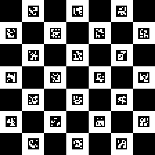
stick it onto a foam board so it’s flat, and take some calibration images with the Raspberry Pi camera. Then feed them to this little script grab the intrinsic matrix and distortion coefficients. There are tons and tons of OpenCV tutorials on this, so I won’t get too much into it, but I will mention that I’ve noticed the higher-order distortion coefficients don’t add much accuracy and can prevent convergence of the calibration optimization, so I have it fix all distortion coefficients but the first to zero. FIXME: check that last link
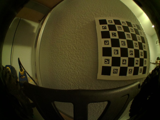
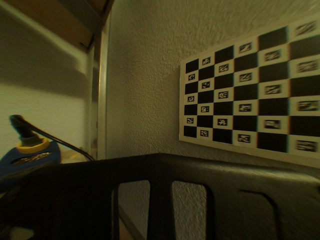
photo of calibration board through fisheye lens
undistored photo
I have another
script which interactively lets me adjust the exact camera angle so that
the floor appears flat and undistorted; there are smarter ways to do this
(namely, place a fixed rectangular object of known size on the floor in front
of the car, take a picture, and use cv2.getPerspectiveTransform to get a
better transformation matrix) but it’s usually good enough.
Then I generate a look-up table which maps each pixel on the screen to a pixel
on the bird’s eye view (this is backwards from cv2.initUndistortRectifyMap
because I had the idea that I wanted to average all the pixels in the source
image that map to a destination pixel… however this is kind of expensive and
doesn’t gain much in practice). The remapped birdseye view is calibrated for 2
cm2/pixel.
The lookup table gets compiled into the C++ code running on the car – the car doesn’t need OpenCV at all.
Camera color spaces
Most camera sensor chips, including the OV5647 in every Raspberry Pi camera, can send images in other color spaces than RGB – in parcular, YUV420 which is what JPEG uses, where two color channels are sent at half resolution. The nice thing about YUV is that it’s a perceptual color space and bold colors used in road markers, signs, and traffic cones can be linearly separated pretty easily.

(image credit: Wikipedia)
To detect yellow lines on a road, the -U channel is usually enough, unless there are also orange objects in which case I subtract a bit of V so orange doesn’t confound the yellow detection. (There isn’t usually anything bright green on the road, but maybe it would be safer to limit that, too)
I find this to be much more useful than, for example, HSV.
Detecting lane markers from birds’ eye view
Now that I have a top-down looking image with a known pixel scale, and I know approximately how wide the lane markers we’re looking for are, I draw an analogy to signal processing – scanning pixels from left to right, there should be a pulse of a certain width and color. Assuming these pulses can’t be too close together, I used matched filter that can be convolved with each row of the image called a “top hat” filter. (I got this idea from a few other papers on the topic but there isn’t one I can specifically point to; if you search for “lane markers” and “top hat filter” it’ll come up)
FIXME YUV -U = Y
The filter kernel is [-1, -1, 2, 2, -1, -1] (it’s called a “top hat” filter because when you plot that it looks like a tall hat). Notice that it sums to 0, so if the image is bright or dark it doesn’t matter, the activation is 0. The maximum activation happens when there’s a two-pixel wide band of yellow with two pixels of not-yellow around it.