My DIYRobocars autonomous RC car has come a long way since my last post on the subject. I want to highlight a localization algorithm I came up with which works really well, at least in this specific setting. I’ve been using it in races for a while and it really stepped up the speeds I was able to achieve without the car getting “lost” – about 22mph on the front straight of this small track. It makes use of a fisheye camera looking towards the ceiling, and a localization update runs in about 1ms at 640x480 on a Raspberry Pi 3, with precision on the order of a few centimeters.

Here is a recent race against another car which is about as fast, except it uses LIDAR to localize using the traffic cones as landmarks. (My car previously localized using the cones as well, except using a monocular camera, but the ceiling lights are much better when we have them. Cone-based localization deserves a blog post of its own.) It’s a three lap head-to-head race where there’s an extra random cone on the track. We haven’t developed passing strategies yet though, so there are frequent racing incidents…

DIYRobocars race on March 7, 2020. We had a little accident but my car (blue) somehow made it through unscathed… I finished my three laps just to record a time for that heat.

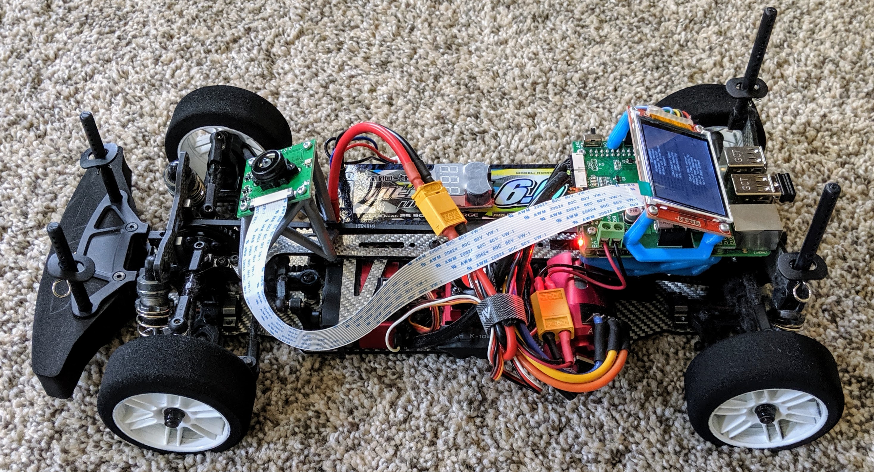
I put a fisheye lens Raspberry Pi camera out the front windshield of a 1/10 scale touring car. It’s mounted sideways because it has a wider field of view horizontally, and I wanted more pixels looking towards the front so I could see a bit of the ground ahead. (Full hardware details are on the github repo.) Here is what it looks like without the lid:

I record telemetry and video in each race, which I can then replay through a Dear ImGui-based tool:

In the lower-right corner of the video is a virtual view of the car’s position and speed, entirely derived from the ceiling light localization algorithm.

With the fisheye lens, it can see a lot of ceiling lights from any point on the track, and they’re all set up in a regular grid with one or two exceptions. The algorithm is robust to extra lights being added, lights being burned out, and other cars flying over the top of the camera (watch closely at 0:07), without losing tracking.

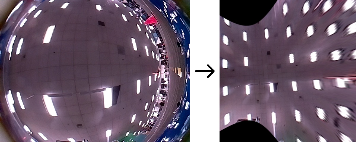
Since it’s hard to tell what’s going on from the raw, sideways fisheye camera, the tool has an option to use cv2.undistort and remap the image as if it were looking straight out the front windshield:

The basic assumptions: ground vehicle localization under a drop ceiling

To make this practical at high FPS on a Raspberry Pi, I chose to make some simplifying assumptions: assume all the ceiling lights are point sources on a perfectly even grid, and that the camera moves along the floor at a fixed height. This turned out to be good enough to work in practice. The method doesn’t necessarily require an even grid, it just needs to be able to determine the distance to the nearest landmark from any point. In a grid, that’s trivial, but it’s not hard to use a map of the ceiling layout instead.

I also assumed I knew the grid size ahead of time, since I can just measure the ceiling tile sizes and count the spaces between lights, and also measure the height of the ceiling from the camera.

Further, the setting allows us to initialize the algorithm approximately at a known location, namely the starting line. If the pattern of lights is perfectly regular, there’s no way to tell which grid cell you started in, so we have to assume we’re at the one containing the start of the race when we reset our state.

Camera model

The first step is to deal with the lens distortion. This is particularly obvious when using a fisheye lens, but every lens should be calibrated. OpenCV provides a module for calibrating converting from distorted/undistorted fisheye coordinates.

I won’t go too much into camera calibration here, but what I do is print this ArUco calibration target, take still photos of it from several angles, and use this script to get the camera intrinsic parameters.

With those parameters, you can use several OpenCV utilities to do things like undistort images (shown above) or compute ideal pinhole camera ray vectors from each pixel with cv2.undistortPoints.

In my tracking code, the initialization step computes a lookup table with the supplied camera parameters. For each pixel, the lookup table has a \(\left[x, y, 1\right]\) vector which forms a ray in 3D space starting at the camera and heading out towards the ceiling. There is also a circular mask to filter out pixels pointing too far away from the ceiling.

Note that the tracking code does not use cv2.undistortImage or equivalent. The illustration above shows what undistorting the whole image does: objects far away from the camera with relatively small numbers of pixels in the source image take up a large number of blurry pixels in the output, and the objects directly in front taking up most of the image are a small portion of the output. What I want to do is give equal weight to each pixel in the source image, and less weight to potential outliers. That way, the lights directly above the camera are mostly what it will try to track on, which gives better accuracy.

Once the lookup table is available, the problem reduces to matching a 2D grid to all the corrected pixel locations for all pixels within the mask which look like ceiling lights, meaning the grayscale pixel is brighter than some threshold. The mask is necessary to deal with reflections from the car’s body and light from nearby windows – it makes sure we’re only looking upwards for ceiling lights.

Least squares grid alignment

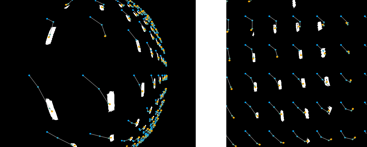
Grid alignment objective. Blue dots: initial uninitialized configuration \([u, v, \theta] = (0, 0, 0)\); orange dots: fit after five iterations of the Levenberg-Marquardt algorithm described below. Left: the grid dots are transformed back into the fisheye distortion here to show the fit on the original image. Right: the fit in undistorted space.

We can solve this with the same hammer we pound on all the other nails with in computer vision: nonlinear least squares via Levenberg-Marquardt, which is a fancy name for the ordinary least squares algorithm with a simple tweak to make sure it converges.

The vehicle state is defined as \([u, v, \theta]\) where \(u, v\) are the position within the grid along the \(x\) and \(y\) axes respectively, and \(\theta\) is the heading angle of the vehicle. We’ll also define \(x_{spc}\) and \(y_{spc}\) as the grid spacing in each axis.

Conceptually, if we superimpose a grid with that spacing on the ceiling, rotate it by \(-\theta\) around the center and then translate it by \([-u, -v]\), the grid should line up with the pixels in our image which are above the “white” threshold.

To do the optimization, we start with an initial guess for \([u, v, \theta\)] and repeat two steps: First, find the nearest grid point to every transformed white pixel, and then solve for an updated \([u, v, \theta]\) to minimize the residuals. Solving for \([u, v, \theta]\) may cause some pixels to match different grid points, so repeating the two steps a few times is usually necessary, otherwise it would be solved in closed form. In practice, once the algorithm is “synced up”, only two iterations are really necessary to keep up with tracking.

Let’s define a residual for every undistorted white pixel \([x_i, y_i]\) measuring the distance to the closest grid point \([g_{xi}, g_{yi}]\):

This says: Rotate each pixel \([x_i, y_i]\) by the car’s heading angle \(\theta\), subtract the car’s position \([u, v]\), and compare it to the grid point we think it should be on \([g_{xi}, g_{yi}]\). We want to minimize the sum of the squares of all residuals, \(\sum_{i} \mathbf{r}_{i}^\top \mathbf{r}_i\).

(Note: \([x_i, y_i]\) here are the pixels after undoing the camera transform / distortion, so they are not pixel coordinates but rather normalized coordinates. You can think of it as a ray shooting from the camera intersecting a plane 1 unit in front of the camera; (1, 0) would thus be a ray 45-degree angle to the right of center shooting out of the camera.)

If we’re fitting to a grid, then \([g_{xi}, g_{yi}]\) can be found simply by taking the transformed point modulo the grid spacing \(x_{spc}, y_{spc}\). In principle, any pattern of landmarks, not just grids, can be used here.

Here’s my Python prototype implementation that finds the nearest grid point:

def moddist(x, q):
    return (x+q/2)%q - q/2

def nearest_grid(xi, yi, xspc, yspc):
    gxi = moddist(xi, xspc)
    gyi = moddist(yi, yspc)
    return gxi, gyi

To do the least-squares minimization, we need to compute the Jacobian (a fancy word for the derivative of a vector with respect to a vector) of the residuals, which is simple enough. I used SymPy in a Jupyter notebook:

from sympy import *
init_printing()

x, y, gx, gy = symbols("x_i y_i g_x_i g_y_i")
u, v, theta = symbols("u v theta")
S, C = sin(theta), cos(theta)
R  = Matrix([[C, -S], [S, C]]).T
uv = Matrix([[u], [v]])
xy = Matrix([[x], [y]])
gxy = Matrix([[gx], [gy]])
r = R*xy - uv - gxy
r

J = r.jacobian(Matrix([[u, v, theta]]))
J

Now, to actually compute our least squares update, we need to compute \(\delta = \left(\sum_i \mathbf{J}_i^\top \mathbf{J}_i + \lambda \mathbf{I} \right)^{-1} \left(\sum_i \mathbf{J}_i^\top \mathbf{r}_i\right)\). Looks complicated, but what it means is we need to add a up contribution for each pixel into a symmetric matrix and a vector, and then solve for an update to \([u, v, \theta]\). \(\lambda\) is effectively a hyperparameter of the algorithm which keeps the matrix from becoming singular. I just set it to 1 and never really needed to tune it afterward. (I tried setting it to 0, making this the Gauss-Newton iteration, but that will diverge if there aren’t enough observations, like when something covers the camera for exmaple).

Our Jacobian is pretty sparse, though, so let’s see what those terms look like:

simplify(J.T*J)

SymPy’s simplify was smart enough to reduce the bottom right entry which was the length of a vector rotated about \(\theta\) to just the length of the vector, as rotation wouldn’t affect the length. So to compute this, we need to sum up rotated versions of each white pixel and the squared distance from the center.

Now, that was the Jacobian for just one pixel. For convenience, let’s define a couple auxiliary variables to clean that up a bit:

These are the partial derivatives of \([x_i, y_i]\) rotated by \(\theta\).

If we add up all the pieces we need, our final left-hand term is:

In the end, to compute this, we only need to calculate the three running sums in the right column (or bottom row) of the matrix, and to count up the number of white pixels \(N\).

Now, the right hand side is a bit messier, so let’s assume we’ve already computed the residuals (the distance of each white pixel from the grid point it belongs to):

We’ll also assume we computed \(\delta R x_i\) and \(\delta R y_i\) and swap in our simpler Jacobian for J.

dx, dy = symbols("\Delta\\ x_i \Delta\\ y_i")
dRx, dRy = symbols("\delta\\ Rx_i \delta\\ Ry_i")
J_simple = Matrix([[-1, 0, -dRx], [0, -1, -dRy]])
r_simple = Matrix([[dx], [dy]])
J_simple.T*r_simple

Again, this is the contribution from a single pixel; to get the final term we need to solve it, we have to sum up \(\mathbf{J}^\top\mathbf{r}\):

If you’re actually following along this far, I salute you! We’re almost done deriving what we need to get a working algorithm.

Adding it all up

To recap, we’re starting from an initial guess of our grid alignment \([u, v, \theta]\), and we’re doing a nonlinear least squares update to improve our fit. The things we need to compute to solve it are a few different sums, added up over each pixel \([x_i, y_i]\) brighter than the threshold to consider it part of a ceiling light. They are:

These are just six floats we add up while looping over the image pixels, and then we construct and solve this system of equations for our update:

\(\begin{bmatrix}u' \\ v' \\ \theta'\end{bmatrix} = \begin{bmatrix}u \\ v \\ \theta\end{bmatrix} - \begin{bmatrix} N + \lambda & 0 & \Sigma_1 \\ 0 & N + \lambda & \Sigma_2 \\ \Sigma_1 & \Sigma_2 & \Sigma_3 + \lambda \end{bmatrix}^{-1} \begin{bmatrix} -\Sigma_4 \\ -\Sigma_5 \\ -\Sigma_6 \end{bmatrix}\)
Yes, those minus signs are redundant, but I’m keeping it in the original Levenberg-Marquardt form

Solving the system

It would be relatively easy and fast at this point to use a linear algebra package to solve this. My Python prototype implementation just constructed these matrices and called np.linalg.solve here, which is definitely the way to go in Python.

But when porting it to C++, I considered using Eigen before wondering whether it was even worth using for a 3x3 matrix solve. What would happen, I wondered, if I just had SymPy spit out a solution?

# redefine our JTJ, JTr matrices in terms of the sums defined above
N, S1, S2, S3, S4, S5, S6 = symbols(
    "N Sigma1 Sigma2 Sigma3 Sigma4 Sigma5 Sigma6")
# Note: we'll add lambda to N and S3 before computing the solution,
# as it simplifies the following algebra a lot.
JTJ = Matrix([[N, 0, S1], [0, N, S2], [S1, S2, S3]])
JTr = Matrix([[-S4], [-S5], [-S6]])
JTr = Matrix([[-S4], [-S5], [-S6]])
simplify(JTJ.inv() * JTr)

Now I know what you’re thinking: “you’re kidding, right?” Are we going to type all that in instead of just using a matrix solver?

Let me show the hidden superpower of SymPy: cse, the common subexpression elimination function. SymPy can also print C code from any expression. cse returns a list of temporary variables and a list of expressions in terms of those variables, generating a very efficient routine for computing ridiculously complex expressions. Check this out:

ts, es = cse(JTJ.inv() * JTr)
for t in ts:  # output each temporary variable name and C expression
    print('float', t[0], '=', ccode(t[1]) + ';')
print('')
for i, e in enumerate(es[0]):  # output C expressions
    print(["u", "v", "theta"][i], '-=', ccode(e) + ';')

float x0 = pow(Sigma1, 2);
float x1 = -x0;
float x2 = N*Sigma3;
float x3 = pow(Sigma2, 2);
float x4 = x2 - x3;
float x5 = 1.0/(x1 + x4);
float x6 = Sigma6*x5;
float x7 = 1.0/(pow(N, 2)*Sigma3 - N*x0 - N*x3);
float x8 = Sigma5*x7;
float x9 = Sigma1*Sigma2;
float x10 = Sigma4*x7;

u -= Sigma1*x6 - x10*x4 - x8*x9;
v -= Sigma2*x6 - x10*x9 - x8*(x1 + x2);
theta -= -N*x6 + Sigma1*Sigma4*x5 + Sigma2*Sigma5*x5;

Once we’ve summed up our Sigma1..Sigma6 variables, the above snippet computes the amount to subtract from u, v, and theta to get the new least squares solution, without needing to call out to a matrix library. It’s really not much code. (I would personally change all pow(x, 2) into x*x first, though).

One thing I glossed over: I took \(\lambda\) out temporarily from the derivation to simplify, so to put it back in you need to do N += lambda; Sigma3 += lambda; before running the above code.

The full algorithm

Let’s put it all together now for the full algorithm.

Initialization

First, calibrate the camera and compute a lookup table equivalent to doing cv2.fisheye.undistort() on all pixels in the image. OpenCV wants sort of a weird matrix shape, so I use something like:

K = np.load("camera_matrix.npy")
dist = np.load("dist_coeffs.npy")

# I calibrated in 2592x1944, but use 640x480 on the car, so compensate
# by dividing the focal lengths and optical centers
K[:2] /= 4.05

# generate a (480, 640, 2)-shaped matrix where each element contains
# its own x and y coordinate
uv = np.mgrid[:480, :640][[1, 0]].transpose(1, 2, 0).astype(np.float32)
pts = cv2.fisheye.undistortPoints(uv, K=K, D=dist)

I further rotate and renormalize pts to compensate for the tilt of the camera, and then export it as a lookup table; the C++ code then loads it on initialization. Let’s call it float cameraLUT[640*480][2].

We’ll also initialize float u=0, v=0, theta=0;

Update from camera image

Step by step, the update algorithm is:

• Get the grayscale image – I have the camera sending native YUV420 frames, so I just take the Y channel here.
• Clear a vector of white pixel undistorted ray vectors xybuf
• For every pixel in the image > the white threshold:
  • Look up cameraLUT for that pixel and push it onto xybuf
• For each solver iteration (I use two iterations):
  • Initialize float accumulators Sigma1..Sigma6 (defined above) to 0
  • Precompute \(\sin \theta\) and \(\cos \theta\) – constant for all pixels
  • For each pixel x, y in xybuf:
    • Compute the distance to the nearest landmark \(\Delta x_i, \Delta y_i\), using e.g. moddist for grids, as well as \(\delta R x_i, \delta R y_i\), etc.
    • Add the pixel’s contribution to Sigma1..Sigma6, defined above in the “Adding it all up” section
  • Compute updates to u, v, theta defined above using the length of xybuf for N.

The actual code running on the car for this is here but it’s a bit cluttered because there are two SIMD versions (SSE and NEON) and a bunch of other optimizations and hacks, and the variable names are a bit different than described in this article, but it should be recognizable from this description.

Efficiently implemented, the most expensive part of this algorithm is the branch misprediction penalty it incurs when thresholding white pixels and adding to xybuf.

Further applications

Making a map of the floor by tracking the motion of the ceiling

In order to actually use this for racing, I need to get a map of the track with respect to the ceiling. This is why I have the camera partially looking towards the floor in front of the car. Here, two masks are defined for the image: one for ceiling-facing pixels, and one for pixels intersecting the floor within a range of distances (not too close, or it will see the hood, and not too far, or it will just be a blur). Using the position and angle of the tracking result, the floor pixels are reprojected to a bird’s eye view as I drive the car around manually along the track.

The tracking isn’t perfect, and the geometry I’m using to project the floor in front of the car isn’t perfect, so there’s a little wonkiness in the result, but it’s good enough to use as a map.

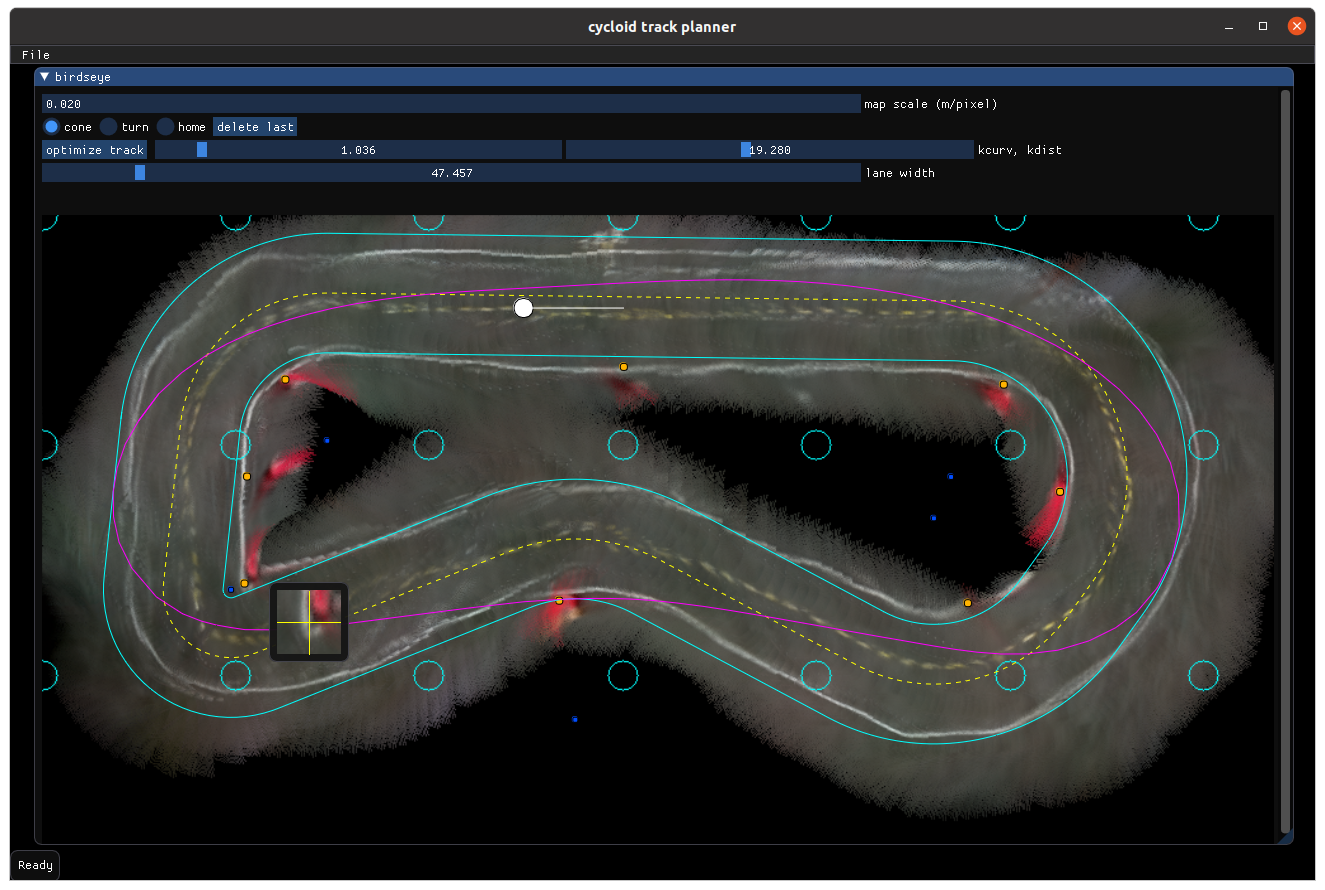
Track planner GUI. Cyan circles are ceiling light locations; blue dots are centers of curvature, orange dots are cone locations. The magenta line is a minimum curvature line, but not one used for racing anymore.

I then import this into another tool to define a racetrack using the ceiling-derived map, run an optimization procedure which computes the best racing line from any point, and send the optimized map to the car. After that, it will drive autonomously.

Conclusion

This ceiling light tracking algorithm works so well I consider localization on this track a solved problem and have been focusing on other areas, like reinforcement learning based algorithms for autonomous racing.

Unfortunately, Circuit Launch, our regular racing venue, has torn out the entire ceiling in a recent renovation, so once we can start racing again we’ll have to see whether the perfect grid assumption still holds, or if it needs to be extended with an actual ceiling map. Nevertheless, I’m pretty confident that this is the best way to do 2D indoor localization.